Building a Multi-Layer Perceptron for FEM Predictions - AI Portfolio Project
This is a portfolio project where I built my first neural network from scratch - a Multi-Layer Perceptron (MLP) that predicts engineering simulation results. Here’s what I learned and the steps I took to build it.
Project Overview
Goal: Build a Multi-Layer Perceptron (MLP) neural network that predicts fracture mechanics results for cracked structures—specifically, whether a crack will grow and cause failure.
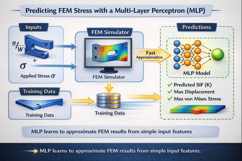
The Engineering Problem: Traditional Finite Element Method (FEM) simulations can take hours to days to analyze crack behavior in structures. This project creates a neural network surrogate model that predicts the same results in milliseconds.
What is FEM? The Lego Analogy
Imagine you want to understand how a rubber ball squishes when you press on it. The physics of a curved, squishy object is incredibly complex. But here’s the trick:
- Divide the ball into tiny pieces (like Lego blocks)
- Apply simple physics to each piece
- Connect all the pieces and see what happens
This is FEM in a nutshell—break complex objects into simple pieces (finite elements), solve each piece, and combine the results.
The Trade-off: More Accuracy = More Time
| Number of Elements | Accuracy | Time |
|---|---|---|
| 100 | Rough | Seconds |
| 10,000 | Good | Minutes |
| 1,000,000 | Excellent | Hours |
| 100,000,000 | Perfect | Days to Weeks |
For complex designs—airplane wings, car crash simulations, cracked structures—you need millions of elements. And that means waiting. A lot.
The AI Solution: Learn Once, Predict Forever
Instead of running expensive FEM simulations every time, what if AI could learn from thousands of previous simulations and predict new results instantly?
Think of it like a chef:
- Traditional FEM = Making every dish from scratch (slow but accurate)
- AI Surrogate = A chef who’s made 10,000 similar dishes and knows the patterns (fast and good enough)
Physics-Informed Training Data: For this learning project, I didn’t have access to real FEM simulation data or expensive commercial software. Instead, I used the Tada-Paris-Irwin formula—a well-established analytical equation from fracture mechanics that calculates stress intensity factors based on crack geometry and loading conditions.
By generating synthetic training data from this physics-based formula, I could:
- Create 5,000+ training examples instantly (no need for real FEM data)
- Learn neural network fundamentals without expensive software licenses
- Ensure the neural network learns physically correct relationships
- Focus on the ML implementation rather than data collection
This approach is a form of Physics-Informed Neural Networks (PINNs)—where the AI learns from known physics laws embedded in the training data. While real-world applications would use actual FEM simulation data, this physics-based synthetic data was perfect for learning how to build and train neural networks for engineering problems.
Why this project?
- Learn neural network fundamentals through hands-on implementation
- Explore physics-informed machine learning (PINN concepts)
- Apply ML to a real engineering problem (not just toy datasets)
- Build a complete ML application (model + API + UI + deployment)
- Create a portfolio piece demonstrating end-to-end ML skills
Tech Stack: Python, PyTorch, FastAPI, React + TypeScript, Docker
Repository: github.com/anachary/mvp-fem-surrogate-engine
Understanding the Problem
The neural network needs to learn this relationship:
Inputs (5 features):
- W: Plate width (mm)
- H: Plate height (mm)
- a: Crack length (mm)
- σ: Applied stress (MPa)
- K_IC: Fracture toughness (MPa√mm)
Outputs (3 predictions):
- K_I: Mode-I Stress Intensity Factor (measures crack severity)
- K_II: Mode-II Stress Intensity Factor (shear mode)
- Safety Factor: Is the structure safe? (K_IC / K_I)
Step 1: Understanding Multi-Layer Perceptron (MLP)
An MLP is the simplest type of neural network. It’s called “multi-layer” because it has:
- Input layer: Takes your data (5 features in our case)
- Hidden layers: Process the data through mathematical transformations
- Output layer: Produces predictions (3 values in our case)
Here’s my MLP architecture:
Input Layer (5)          Hidden Layers              Output Layer (3)
    │                                                      │
    W ─────┐                                               ├── K_I
    H ─────┤                                               │
    σ ─────┼──→ [64 neurons] → [64] → [64] ────────────→  ├── K_II
  K_IC ────┤                                               │
    α ─────┘                                               └── Safety Factor
Why this architecture?
- 3 hidden layers with 64 neurons each: Simple enough to train quickly, complex enough to learn patterns
- Total parameters: ~9,000 (very lightweight!)
- Activation function: Tanh (helps with smooth gradients)
- No dropout or fancy tricks: Keep it simple for learning
Step 2: Building the MLP in PyTorch
Here’s the actual code I wrote for the neural network:
import torch
import torch.nn as nn

class FEMSurrogate(nn.Module):
    def __init__(self, input_dim=5, output_dim=3, hidden_dims=[64, 64, 64]):
        super().__init__()

        # Build the layers
        layers = []
        prev_dim = input_dim

        # Hidden layers
        for hidden_dim in hidden_dims:
            layers.append(nn.Linear(prev_dim, hidden_dim))
            layers.append(nn.Tanh())  # Activation function
            prev_dim = hidden_dim

        # Output layer
        layers.append(nn.Linear(prev_dim, output_dim))

        self.network = nn.Sequential(*layers)

    def forward(self, x):
        return self.network(x)
What’s happening here?
nn.Linear: Creates a fully connected layer (each neuron connects to all neurons in next layer)nn.Tanh(): Activation function that adds non-linearity (helps learn complex patterns)nn.Sequential: Chains all layers togetherforward(): Defines how data flows through the network
Step 3: Preparing the Training Data
Neural networks learn from examples. I needed data showing the relationship between inputs and outputs.
Option 1: Generate Synthetic Data (What I Started With)
I used the Tada-Paris-Irwin formula - a mathematical formula from fracture mechanics:
\[K_I = \sigma \sqrt{\pi a} \cdot F(\alpha)\]Where $\alpha = a/W$ (crack ratio) and:
\[F(\alpha) = 1.12 - 0.231\alpha + 10.55\alpha^2 - 21.72\alpha^3 + 30.39\alpha^4\]This let me generate 5,000 training examples instantly:
python scripts/generate_data.py --synthetic -n 5000
Why synthetic data?
- Fast to generate (no waiting for simulations)
- Perfect for learning and testing
- Can create as many examples as needed
Option 2: Real FEM Data (For Better Accuracy)
Later, I integrated real FEM solver (FEniCSx) to get more realistic data:
python scripts/generate_data.py --fem -n 100
The data is saved in a simple format:
# Data structure
{
    'W': [50, 60, 70, ...],           # Plate widths
    'H': [100, 120, 140, ...],        # Plate heights
    'sigma': [100, 150, 200, ...],    # Applied stress
    'K_IC': [1500, 1600, ...],        # Fracture toughness
    'alpha': [0.2, 0.3, ...],         # Crack ratios
    'K_I_fem': [523, 645, ...],       # Target outputs
    'K_II_fem': [0, 0, ...],          # Target outputs
    'SF_fem': [2.87, 2.48, ...]       # Target outputs
}
Step 4: Training the Neural Network
This is where the magic happens! The network learns by:
- Making predictions
- Comparing predictions to actual values
- Adjusting weights to reduce errors
- Repeating thousands of times
Here’s my training code:
import torch.optim as optim

# Initialize the model
model = FEMSurrogate(input_dim=5, output_dim=3, hidden_dims=[64, 64, 64])

# Loss function: Mean Squared Error
criterion = nn.MSELoss()

# Optimizer: Adam (adjusts weights during training)
optimizer = optim.Adam(model.parameters(), lr=0.001)

# Training loop
for epoch in range(500):
    # Forward pass: make predictions
    predictions = model(train_inputs)

    # Calculate loss: how wrong are we?
    loss = criterion(predictions, train_targets)

    # Backward pass: calculate gradients
    optimizer.zero_grad()
    loss.backward()

    # Update weights
    optimizer.step()

    if epoch % 50 == 0:
        print(f"Epoch {epoch}, Loss: {loss.item():.4f}")
Key concepts I learned:
- Loss function (MSE): Measures how wrong the predictions are
- Optimizer (Adam): Smart algorithm that adjusts weights
- Learning rate (0.001): How big the weight adjustments are
- Epochs (500): Number of times to go through all training data
- Backpropagation: How the network learns (calculates gradients)
Running the Training
I made it simple with a command-line script:
# Train the model
python scripts/train_surrogate.py --train data/fem_synthetic.npz --epochs 500
Training results:
- Time: ~3-5 minutes on CPU
- Final loss: ~0.001 (very low = good predictions!)
- Model saved to:
checkpoints/surrogate_best.pt
The script automatically:
- Splits data into training (80%) and validation (20%)
- Normalizes inputs/outputs for stable training
- Saves the best model based on validation loss
- Stops early if loss stops improving
Step 5: Making Predictions (Inference)
Once trained, using the model is simple:
# Load the trained model
model = FEMSurrogate()
model.load_state_dict(torch.load('checkpoints/surrogate_best.pt'))
model.eval()  # Set to evaluation mode

# Make a prediction
input_data = torch.tensor([[50.0, 100.0, 10.0, 100.0, 1500.0]])  # W, H, a, σ, K_IC
prediction = model(input_data)

# Results
K_I = prediction[0][0].item()      # 523.45
K_II = prediction[0][1].item()     # 0.0
safety_factor = prediction[0][2].item()  # 2.87
Prediction speed: ~0.1 milliseconds on CPU!
Step 6: Building the REST API
To make the model accessible, I built a FastAPI backend:
from fastapi import FastAPI
from pydantic import BaseModel

app = FastAPI()

class PredictionRequest(BaseModel):
    W: float
    H: float
    a: float
    sigma: float
    K_IC: float

@app.post("/predict-crack-sif")
def predict(request: PredictionRequest):
    # Prepare input
    input_tensor = torch.tensor([[
        request.W, request.H, request.a,
        request.sigma, request.K_IC
    ]])

    # Make prediction
    with torch.no_grad():
        output = model(input_tensor)

    return {
        "K_I": output[0][0].item(),
        "K_II": output[0][1].item(),
        "safety_factor": output[0][2].item()
    }
Run the API:
uvicorn src.api.app:app --reload
Test it:
curl -X POST http://localhost:8000/predict-crack-sif \
  -H "Content-Type: application/json" \
  -d '{"W": 50, "H": 100, "a": 10, "sigma": 100, "K_IC": 1500}'
Step 7: Building the Frontend
I created a React TypeScript UI for easy interaction:
- Input sliders for all parameters
- Real-time predictions as you adjust values
- Color-coded safety warnings (green/yellow/red)
- Visualization of results
Step 8: Docker Deployment
Everything packaged in Docker for easy deployment:
# Start the full stack (API + UI)
docker-compose up --build -d

# Access:
# - UI:  http://localhost:3000
# - API: http://localhost:8000
Project Results
Performance:
- Training time: ~3-5 minutes on CPU
- Prediction time: ~0.1 milliseconds
- Model size: ~36 KB
- Accuracy: < 5% error on validation data
What I achieved:
- ✅ Built my first neural network from scratch
- ✅ Learned PyTorch fundamentals
- ✅ Understood backpropagation and gradient descent
- ✅ Created a full-stack ML application
- ✅ Deployed with Docker
Key Learnings
1. MLPs are Simple but Powerful
You don’t need complex architectures for many problems. A simple 3-layer MLP with 64 neurons each can learn complex patterns effectively.
2. Data Preparation is Critical
- Normalize inputs/outputs (makes training stable)
- Split into train/validation sets (prevents overfitting)
- Start with synthetic data (fast iteration)
- Validate with real data (ensures accuracy)
3. Training is Iterative
My first model didn’t work well. I learned to:
- Adjust learning rate (too high = unstable, too low = slow)
- Monitor validation loss (detect overfitting)
- Use early stopping (save best model)
- Experiment with architecture (layers, neurons, activation functions)
4. Deployment Makes it Real
Building the API and UI transformed this from a learning exercise into a usable tool. This taught me:
- FastAPI for serving ML models
- React for building interfaces
- Docker for packaging everything
- REST API design
What’s Next?
I’m planning to extend this project:
- Try different architectures (deeper networks, skip connections)
- Implement uncertainty quantification
- Add more complex crack geometries
- Integrate with real FEM software
- Optimize for mobile deployment
How to Run This Project
The complete code is on GitHub: github.com/anachary/mvp-fem-surrogate-engine
Quick Start (3 steps):
# 1. Generate training data
python scripts/generate_data.py --synthetic -n 5000

# 2. Train the MLP
python scripts/train_surrogate.py --train data/fem_synthetic.npz --epochs 500

# 3. Run the API
uvicorn src.api.app:app --reload
Or use Docker:
docker-compose up --build -d
# UI at http://localhost:3000
# API at http://localhost:8000
Project Structure
mvp-fem-surrogate-engine/
├── src/
│   ├── core/
│   │   ├── surrogate.py          # MLP model definition
│   │   ├── simple_trainer.py     # Training loop
│   │   └── physics_losses.py     # Tada-Paris-Irwin formula
│   └── api/
│       └── app.py                # FastAPI server
├── scripts/
│   ├── generate_data.py          # Data generation
│   └── train_surrogate.py        # Training script
├── ui/                           # React frontend
└── checkpoints/                  # Saved models
Technologies Used
- PyTorch: Neural network framework
- NumPy: Data manipulation
- FastAPI: REST API framework
- React + TypeScript: Frontend
- Docker: Containerization
Conclusion
This project taught me the fundamentals of neural networks through hands-on implementation:
Core ML Concepts:
- Multi-Layer Perceptron architecture
- Forward and backward propagation
- Loss functions and optimization
- Training, validation, and testing
- Model deployment
Practical Skills:
- PyTorch for building neural networks
- Data preparation and normalization
- Hyperparameter tuning
- Building ML APIs with FastAPI
- Full-stack ML application development
Key Takeaway: You don’t need complex models or massive datasets to build useful ML applications. A simple MLP with good data and proper training can solve real-world problems effectively.
Want to learn more about my AI projects? Check out my other posts on neural networks and machine learning.
Project Repository: github.com/anachary/mvp-fem-surrogate-engine
References and Research Papers
This project was inspired by cutting-edge research in physics-informed machine learning and surrogate modeling:
Physics-Informed Neural Networks (PINNs)
-
Raissi, M., Perdikaris, P., & Karniadakis, G. E. (2019) Physics-informed neural networks: A deep learning framework for solving forward and inverse problems involving nonlinear partial differential equations Journal of Computational Physics, 378, 686-707. DOI: 10.1016/j.jcp.2018.10.045 Key contribution: Introduced PINNs that incorporate physics laws directly into neural network training.
-
Karniadakis, G. E., Kevrekidis, I. G., Lu, L., Perdikaris, P., Wang, S., & Yang, L. (2021) Physics-informed machine learning Nature Reviews Physics, 3(6), 422-440. DOI: 10.1038/s42254-021-00314-5 Key contribution: Comprehensive review of physics-informed ML approaches.
Neural Operators and Surrogate Models
-
Lu, L., Jin, P., Pang, G., Zhang, Z., & Karniadakis, G. E. (2021) Learning nonlinear operators via DeepONet based on the universal approximation theorem of operators Nature Machine Intelligence, 3(3), 218-229. DOI: 10.1038/s42256-021-00302-5 Key contribution: DeepONet architecture for learning operators (function-to-function mappings).
-
Li, Z., Kovachki, N., Azizzadenesheli, K., Liu, B., Bhattacharya, K., Stuart, A., & Anandkumar, A. (2020) Fourier Neural Operator for Parametric Partial Differential Equations arXiv preprint arXiv:2010.08895. arXiv: 2010.08895 Key contribution: Fourier Neural Operator (FNO) for fast PDE solving.
Fracture Mechanics and Engineering Applications
-
Tada, H., Paris, P. C., & Irwin, G. R. (2000) The Stress Analysis of Cracks Handbook (3rd Edition) ASME Press. Key contribution: Standard reference for stress intensity factor formulas (Tada-Paris-Irwin formula used in this project).
-
Goswami, S., Anitescu, C., Chakraborty, S., & Rabczuk, T. (2020) Transfer learning enhanced physics informed neural network for phase-field modeling of fracture Theoretical and Applied Fracture Mechanics, 106, 102447. DOI: 10.1016/j.tafmec.2019.102447 Key contribution: Application of PINNs to fracture mechanics problems.
Open-Source Tools and Frameworks
-
Lu, L., Meng, X., Mao, Z., & Karniadakis, G. E. (2021) DeepXDE: A deep learning library for solving differential equations SIAM Review, 63(1), 208-228. DOI: 10.1137/19M1274067 Tool: DeepXDE GitHub - Library for physics-informed neural networks.
-
Takamoto, M., Praditia, T., Leiteritz, R., MacKinlay, D., Alesiani, F., Pflüger, D., & Niepert, M. (2022) PDEBench: An Extensive Benchmark for Scientific Machine Learning arXiv preprint arXiv:2210.07182. arXiv: 2210.07182 Tool: PDEBench GitHub - Benchmark datasets for PDE learning.
Additional Resources
- NVIDIA Modulus: Physics-ML framework for simulations - developer.nvidia.com/modulus
- FEniCS Project: Open-source FEM solver - fenicsproject.org
- PyTorch Documentation: Deep learning framework - pytorch.org
Note: This project implements a simplified MLP-based surrogate model with physics-informed training data generation. For more advanced applications, consider exploring the full PINN and neural operator frameworks referenced above.